Modeling Interventions in Causal Bayesian Networks
Learning causal Bayesian Networks from data relies on interventions.

Eaton and Murphy (2007) provide a breakdown of various types of interventions, which I present here in simple form. Modeling interventions refers to an experimenter manipulating one or more variables in order to elucidate the causal relationships between them. The premise is that in order to learn causal relationships between the variables, such interventions are necessary.
In biology, genetic knockouts are an example of an intervention. They are intended to remove the gene’s products from the system entirely, so that the effects of its removal on other proteins becomes apparent.
Interventions vary into two key aspects, which variables they affect and how they affect them. In terms of “which” variables they affect, there are three kinds of interventions: (1) targeted interventions, (2) side-effect interventions, and (3) uncertain interventions.
A targeted intervention has one target variable, and no direct effects on others. An example is an experimental design where a given variable is fixed at different levels.
Side affect interventions also target one variable, but may have unexpected direct effects on other variables. An example is a drug treatment that is designed to inhibit the activity of one protein (the target variable), but has unexpected chemical affects on other proteins (other variables).
With uncertain interventions, it is not known which variables will be directly affected. An example is a genomics experiment where gene expression data is collected from a disease and healthy populations. Disease status is an uncertain intervention, because it is thought to directly influence the expression of some genes (variables in the data), but perhaps it is not known which are affected.
In terms of how the interventions affect the variables, there are two kinds of effects: stochastic and fixed. A fixed intervention fixes a variable to a specific value, such that there is no uncertainty as to what the value of the variable will be when the intervention occurs.
A stochastic intervention allows for uncertainty by, rather than fixing the value, changing the probability distribution of the variable so some values become more or less likely. This can be viewed as a change in the underlying mechanism behind the variable.
Data from experiments with solid statistical experimental design, such as a randomized controlled trial, is extremely powerful in getting to the core of how variables affect one another. Such experimental designs are characterized by having a set of fixed and targeted interventions applied to the explanatory variables.
However, such designs expensive, and often it is not possible or ethical to intervene in all the variables. The Bayesian network framework allows for a more flexible set of interventions, still working with cases where some but not all variables can be targeted for interventions, and where the effects of the interventions can be stochastic and uncertain.
What is the Best Way to Model a Targeted Intervention?
Fixed, targeted interventions can be modeled in 2 ways. The first is by modeling them directly in the score. The score is based on likelihood. In instances of the data where a given node is subject to fixed intervention, the value of the node is 100% certain, and that certainty is incorporated in the likelihood.
The second approach is to model the intervention directly as a node.
The bnlearn package in R, allows incorporation of targeted interventions into a score called the Bayesian Dirichlet equivalent score, which works with categorical variables. The intervention scoring approach is described in Heckerman.
Conceptually, both approaches are equivalent (see Koller’s (2009) discussion on “ideal interventions”. In the context of learning networks from data, the search space is the same, assuming side effects are not allowed. However, it may be the case that the search algorithm that traverses the space of network structure may behave differently in either case. To see if this is the case, in the following analysis I compare both approaches to make sure there don’t differ to severely.
Gaussian Simulation Data
Below, I simulate intervention data from a multivariate Gaussian joint distribution and compare the score and node-based approaches to modeling targeted interventions.
All the code for this write-up is available in this gist, and the R Markdown file used to generate this document is available in Github.
The multivariate Gaussian factorizes into:

The variables are simulated using the following means and standard deviations:
simObservationalData <- function(m){
  a <- data.frame(A = rnorm(m, 1, 1),
               B = rnorm(m, 2, 3),
               C = rep(0, m),
               D = rep(0, m),
               E = rnorm(m, 3.5, 2),
               F = rep(0, m),
               G = rnorm(m, 5, 2))
  a$C <- 2 * (a$A + a$B) + rnorm(m, 2, 0.5)
  a$D <- 1.5 * a$B + rnorm(m, 6, 0.33)
  a$F <- 2 * a$A + a$D + a$E + 1.5 * a$G + rnorm(m, 0, 1)
  return(a)
}
The interventions are simulated by applying a bit of boolean logic. If a variable is the target of intervention, then its distribution is modified to – a very low mean and little variance so the values of the intervention targets are to the far left of the observational values.
simInterventionData <- function(int, m) {
  a <- data.frame(A = rnorm(m, 1, 1),
               B = rnorm(m, 2, 3),
               C = rep(0, m),
               D = rep(0, m),
               E = rnorm(m, 3.5, 2),
               F = rep(0, m),
               G = rnorm(m, 5, 2))
  a[, int] <- rnorm(m, -30, .01)
  if(int != "C") a$C <- 2 * (a$A + a$B) + rnorm(m, 2, 0.5)
  if(int != "D") a$D <- 1.5 * a$B + rnorm(m, 6, 0.33)
  if(int != "F") a$F <- 2 * a$A + a$D + a$E + 1.5 * a$G + rnorm(m, 0, 1)
  return(a)
}
An observational dataset of 5000 replicates is simulated, and one intervention dataset simulating a knockout for each node is simulated, also with 5000 replicates per dataset.
Modeling Side Effect Interventions
Two examples of networks where targeted interventions are modeled as nodes:
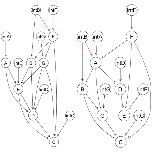
Each normal node has an intervention parent. Intervention nodes are exogenous, fixed variables, and thus are parentless. Between the normal nodes, any directed acyclic graph structure is possible.
Intervention nodes are allowed to affect nodes other than their intended targets. These are side effects. The side effects are demonstrated with the red edges.
Structure Learning Comparison of Targeted and Side Effect Interventions
Graphs are learned via bootstrap resampling. For each bootstrap dataset, the Gaussian data is discretized into categorical data with 3 categories: “low”, “medium”, and “high”. Bayesian network structures are fit using both targeted and node modeling methods. Both methods use tabu search to search the space of graphs, optimizing over log Bayesian Dirichlet equivalent score. In the case of modeling interventions into the score, the score is modified by passing a list of interventions as an argument in the search function (see the code). For each modeling approach, a consensus graph is chosen via model averaging.
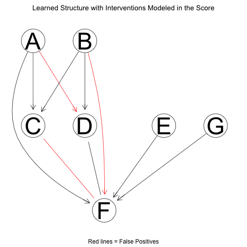
The network structure learned with interventions incorporated into the score is as follows:
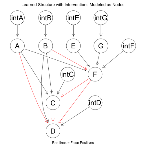
The network structure learned with intervention as nodes is as follows:
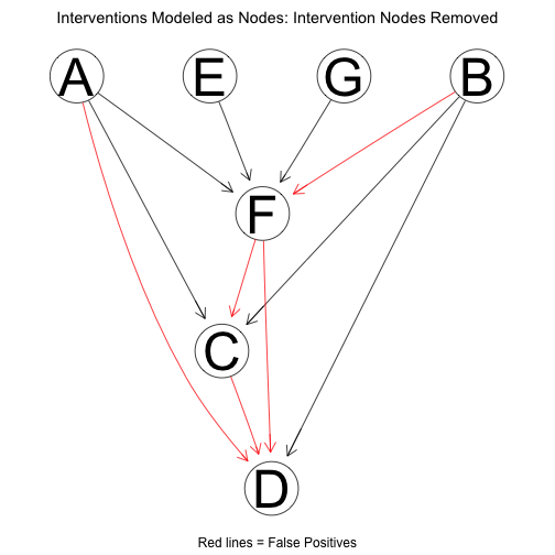
Removing the intervention nodes, the structure reduces to:
Using the package pcalg, the learned network can be compared against the true network. Note that the networks are compared in terms of Markov equivalence (Markov equivalent graphs encode the same conditional independence assumptions though it is possible they have different structure), so the numbers look a bit better than is implied by the above plots. With score-based interventions, performance is as follows:
##    tpr    fpr    tdr
## 1.0000 0.2143 0.7000
When the interventions are incorporated as nodes:
##    tpr    fpr    tdr
## 1.0000 0.2857 0.6364
Despite the instance seen above, when rerunning the algorithm there will be times when one method out performs the other, and others when they tie. In any case the two approaches can produce different results.
Some Negative results
Similar distribution of evaluation statistics across bootstrap samples
The two approaches seem similar in terms of how well the point estimate of the network structure reconstructs the “true” network. What if the performance statistics were more stable for one method than the other? To test this, instead of looking at the performance statistics of the consensus networks, I obtained them to the networks from each bootstrap sample. If the performance statistics had more variation across bootstrap samples with method relative to the other, it would imply the learning results for that method were less stable.
The following is the standard error across bootstrap samples when modeling the interventions in the score:
##     tpr     fpr     tdr
## 0.00000 0.04073 0.02719
The standard errors when interventions are modeled as nodes:
##     tpr     fpr     tdr
## 0.00000 0.02690 0.01958
So it seems there is not much of a difference in variation. There may be a difference with smaller datasets, but I restrict my interest to data rich cases here.
Conclusions
The approaches have comparable results for large data sets. So a practical standpoint, the node based approach is more preferable since it is easier to implement, and can be easily adjusted to allow for side effects, if the targeted assumption seems too restrictive.
References
Radhakrishnan Nagarajan, Marco Scutari, Sophie Lebre. (2013) Bayesian Networks in R with Applications in Systems Biology. Springer, New York. ISBN 978-1461464457.
Marco Scutari (2010). Learning Bayesian Networks with the bnlearn R Package. Journal of Statistical Software, 35(3), 1-22.
Markus Kalisch, Martin Maechler, Diego Colombo, Marloes H. Maathuis, Peter Buehlmann (2012). Causal Inference Using Graphical Models with the R Package pcalg. Journal of Statistical Software, 47(11), 1-26.
Alain Hauser, Peter Buehlmann (2012). Characterization and greedy learning of interventional Markov equivalence classes of directed acyclic graphs Journal of Machine Learning Research, 13, 2409-2464.