Visualizing Signal Flow in Cell Signaling Model
How do you visualize signal flow through a signal transduction pathway?
Take the well-studied MAPK/ERK pathway as an example:
- The signal starts when a ligand binds to a receptor.
- The receptor binding activates Ras
- Ras activates Raf (aka MapKKK)
- Raf activates Mek (MapKK)
- Mek activates Erk (MapK)
- Erk activates the transcription of a gene
Here the flow of signal is Signal -> Ras -> Mek -> Erk -> Response. I downloaded a Map/Erk biochemical model and visualized the reaction graph. The reaction graph connects species (proteins, compounds, etc) to the reactions that involve the species.
Steps to producing reaction graph:
- Download SBML format from biomodels.org
- Import into Cytoscape using the plug-in Petriscape
- Export csv files of network information
- Import csv files into R
- Produce tables of vertices and edges. Download directly: here and here
- Plot in igraph
Code for igraph plotting:
load("huang_mapk_edgelist.R")
load("huang_mapk_vertexlist.R")
library(igraph)
g <- graph.data.frame(edge.list, directed = T, vertices =  mapk.nodes)
## Prepare nodes for plotting
### Use the term "place" for chemical species and "transition" for reactions as is
### consistent with Petri net analysis
V(g)$type <- "place"
V(g)[grep("r", V(g)$name)]$type <- "transition" #grep the reaction nodes and call them "transitions"
V(g)$shape <- "circle"
V(g)[V(g)$type == "transition"]$shape <- "square"
V(g)$color <- "lightblue"
V(g)[V(g)$name == "E1"]$color <- "blue"
V(g)[V(g)$name == "PP_K"]$color <- "red"
#The following is a force-directed layout.
#I generated the following coordinates using Fruchterman-Reingold layout,
#then passed them to plot as a fixed argument for consistency
nice.layout <- matrix(c(84, 112, 20, 181, 201, 244, 280, 271, 328,
                        385, 376, 295, 85, 104, 165, 234, 241, 365,
                        337, 283, 430, 326, 43, 40, 132, 145, 153,
                        61, 164, 176, 199, 292, 278, 255, 220, 209,
                        226, 309, 296, 305, 250, 262, 285, 345, 332,
                        309, 313, 322, 335, 399, 408, 375, 296, 177,
                        220, 259, 371, 337, 195, 81, 109, 161, 51,
                        308, 265, 200, 368, 247, 97, 195, 289, 410,
                        80, 0, 257, 281, 272, 225, 209, 181, 318, 319,
                        320, 359, 357, 368, 290, 285, 212, 252, 251,
                        334, 142, 141, 138, 52, 54, 38, 163, 170, 198,
                        100, 115, 89), ncol=2)
plot.igraph(g, layout = nice.layout, vertex.size =3, vertex.label.dist=-.37,
            edge.arrow.size=.4 )
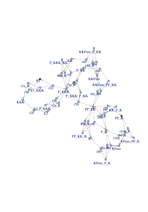
The dark blue node E1 is the source of signal. PP_K (doubly-phosphorylated Erk) is the response.
This reaction graph does not clearly show how signal flows from E1 to PP_K. Generally, reaction graphs do not provide a clear representation of signal flow. In the following, I describe how to manipulate the reaction graph so signal flow becomes clear.
Shortest Path Approach
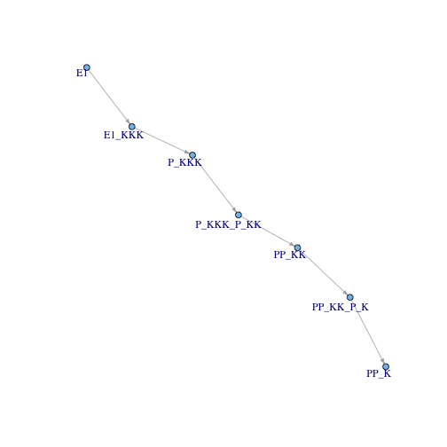
One approach to this problem is to find the shortest path from source to response through the reaction graph. igraph makes this easy:
sp <- get.shortest.paths(g, from = "E1", to = "PP_K", output="epath")$epath[[1]]
directGraph <- suppressWarnings(subgraph.edges(g, sp))
V(directGraph)$label <- V(directGraph)$description
new.layout <- matrix(c(20, 146, 279, 430, 89, 205, 350, 53,
                       115, 176, 239, 313, 387, 410, 266, 126, 0,
                       341, 191, 59, 375, 302, 229, 156, 92, 27), ncol = 2)
plot.igraph(directGraph, layout = new.layout, vertex.size =4, vertex.label.dist=-.37,
            edge.arrow.size=.4 )
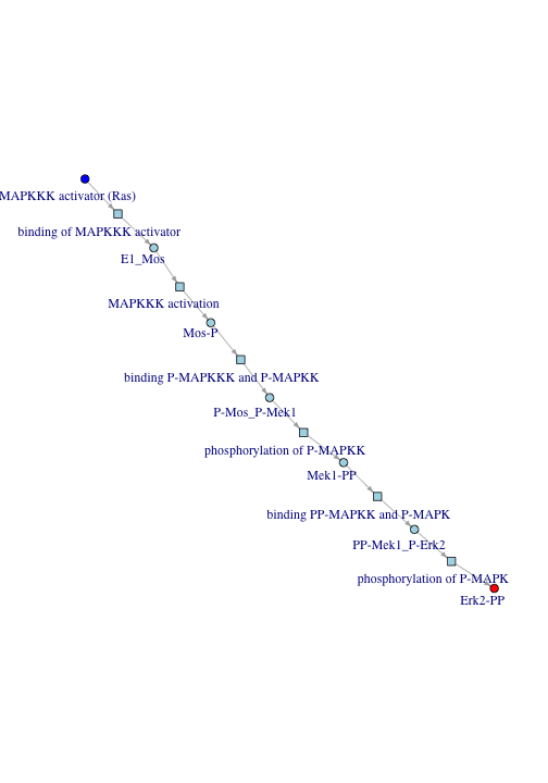
This graph resembles the expected Signal -> Ras -> Mek -> Erk -> Response path. However, what about when there are multiple paths of signal flow? Longer paths can be just as important to overall signal flow as the shortest path. In such cases a different approach is needed.
Subnetwork Approach
Biologists consider the unphosphorylated form of a protein as “inactive”, and the phosphorylated form as “active”. Rather than having two graph nodes for the active and inactive forms of the protein, why not have one “super-node” representing a variable with two states; “active” and “inactive”?
To find which species can be combined into super-nodes, find the null space of the incidence matrix, the matrix of the reaction graph. This provides sets of species whose combined total is conserved, meaning the total does not change as the system changes. The positive elements from the null space vectors provide these sets, called place-invariants. The species in a place-invariant form a super-node.
Similarly, the null space of the transpose of the incidence matrix provides you with transition-invariants. These are sets of reactions that form repeating cycles. The state of the system right after one of these cycles occurs is the same as it was right before it occurred.
The reactions in a cycle (transition-invariant) connect to species, which are members of super-nodes. These connected super-nodes and cycles form subnetworks. Each subnetwork is a step in the flow of the signal.
Petri net theory calls this approach “invariant analysis”. In the age of high-throughput bioinformatics, our knowledge about which proteins interact has grown far faster than our knowledge about the kinetics of those interactions. Invariant analysis provides insights into the workings reaction networks even when reaction rates are not available. The Sackman (2006) reference below has been my go-to source on this type of analysis in the context of signal transduction.
My code for finding invariants starts with finding the null space. Then I find minimal sets of nodes corresponding to positive elements in null space vectors. I use the Null function in the MASS package to calculate the null space:
getMinimalInvariants <- function(S){
  # Get the places and transitions corresponding to minimal invariants of an incidence matrix
  # To get place invariants, use incidence matrix (rows corresponding to places and columns to transitions)
  # To get transition invariants, use transpose of incidence matrix
  # Returns a list where each element is an invariant containing an array of the members of the invariants
  require(MASS, quietly = T)
  nullMat <- round(Null(S), 4)
  rownames(nullMat) <- rownames(S)
  invariants <- list()
  for(j in 1:ncol(nullMat)){
    nullVec <- nullMat[, j]
    valCounts <- table(nullVec)
    valCounts <- valCounts[valCounts != 1]
    valCounts <- valCounts[names(valCounts) != 0] #clear vals that rounded to 0
    valCounts <- valCounts[names(valCounts) > 0] #clear negative elements
    if(length(valCounts) > 0){
      for(i in 1:length(valCounts)){
        val <- valCounts[i]
        invariant <- names(nullVec[nullVec == names(val)])
        invariants <- c(invariants, list(invariant))
      }
    }
  }
  lengths <- sapply(invariants, length)
  invariants <- invariants[order(lengths)]
  if(length(invariants) > 1){
    for(i in 1:(length(invariants) - 1)){
      for(j in (i+1):length(invariants)){
        invariants[[j]] <- setdiff(invariants[[j]], invariants[[i]])
      }
    }
  }
  invariants <- invariants[which(sapply(invariants, length) > 0)]
  invariants
}
Now that I can find invariants, I start with the place-invariants.
places <- V(g)[V(g)$type == "place"]$name
transitions <- V(g)[V(g)$type == "transition"]$name
adjMat <- as.matrix(get.adjacency(g))
pre <- adjMat[places, transitions]
post <- t(adjMat[transitions, places])
S <- post - pre
pInvariants <- getMinimalInvariants(S)
Next, I can apply biological interpretation to each place-invariant. I can see here that each invariant corresponds to different levels of activity (phosphorylations, indicated by “P”) for a given species. With that knowledge I can give each place-invariant a convenient name.
names(pInvariants) <- c("Mek-Erk", "Erk-Phosphotase", "Raf", "Raf-Mek", "Mek-Phosphotase", "Mek", "Erk")
pInvariants


## $`Mek-Erk`
## [1] "PP_KK_K"   "PP_KK_P_K"
##
## $`Erk-Phosphotase`
## [1] "KPase_PP_K" "KPase_P_K"
##
## $Raf
## [1] "KKK"   "P_KKK"
##
## $`Raf-Mek`
## [1] "P_KKK_KK"   "P_KKK_P_KK"
##
## $`Mek-Phosphotase`
## [1] "KKPase_PP_KK" "KKPase_P_KK"
##
## $Mek
## [1] "KK"    "P_KK"  "PP_KK"
##
## $Erk
## [1] "K"    "P_K"  "PP_K"
Moving on to the transition-invariants, see what happens when I plot both the place and transition-invariants together:
drawGraphWithInvariants <- function(graph, g.layout){
  #Did this as a function so I could apply to multiple graphs
  #Takes in a graph as described above, with a type attribute labeled "place" or "transition"
  places <- V(graph)[V(graph)$type == "place"]$name
  transitions <- V(graph)[V(graph)$type == "transition"]$name
  ## Get adjacency
  adjMat <- as.matrix(get.adjacency(graph))
  ## Incidence matrix is derived by taking reactant - reaction relationship matrix
  ## and product - reaction relation matrix and subtracting former from latter.
  pre <- adjMat[places, transitions]
  post <- t(adjMat[transitions, places])
  S <- post - pre
  # Invariant calculation matrix
  pInvariants <- getMinimalInvariants(S)
  tInvariants <- getMinimalInvariants(t(S))
  # Name them
  names(pInvariants) <- unlist(lapply(pInvariants, function(p) paste(p, collapse = "--")))
  names(tInvariants) <- unlist(lapply(tInvariants, function(t) paste(t, collapse = "--")))
  # Label nodes in the graph
  require(reshape, quietly=TRUE)
  invariantMap <- rbind(melt(pInvariants), melt(tInvariants))
  names(invariantMap) <- c("name", "invariant")
  rownames(invariantMap) <- as.character(invariantMap$name)
  V(graph)$invariant <- invariantMap[V(graph)$name, "invariant"]
  invariantVertex <- lapply(c(pInvariants, tInvariants), function(inv){
    V(graph)[V(graph)$name %in% inv]
  })
  V(graph)$color <- "lightblue"
  V(graph)[is.na(V(graph)$invariant)]$color <- "pink"
  V(graph)[V(graph)$name == "E1"]$color <- "blue"
  V(graph)[V(graph)$name == "PP_K"]$color <- "red"
  plot.igraph(graph, layout = g.layout, vertex.size =3, vertex.label.dist=-.37,
              edge.arrow.size=.4, mark.groups=invariantVertex)
}
drawGraphWithInvariants(g, nice.layout)
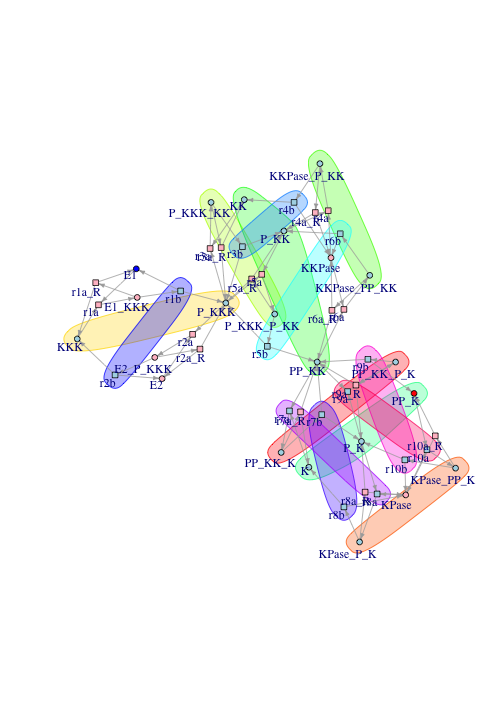
Nodes not involved in any invariant are colored pink in the plot.
There is a problem with the transition-invariants in the plot. Many of the reactions belong to no invariant at all. This is wrong because signals only travel though reactions belonging to transition-invariants and species connected to those reactions.
The problem is the network contains reversible reactions. Many of the reactions in cell signaling are indeed reversible, for example two species can bind and then unbind again. The forward and reverse reactions cancel each other out, resulting in zero entries in the incidence matrix, affecting calculation of the null space.
In applying invariant analysis to signaling networks, this is remedied by removing the reverse reactions. These are conveniently labeled with the suffix “R” in the reaction graph. When the reverse reactions are removed, the transitions form transition-invariants:
reverse.nodes <- grepl("R", V(g)$name)
subg <- suppressWarnings(igraph::subgraph(g, V(g)[!reverse.nodes]))
drawGraphWithInvariants(subg, nice.layout[!reverse.nodes, ])
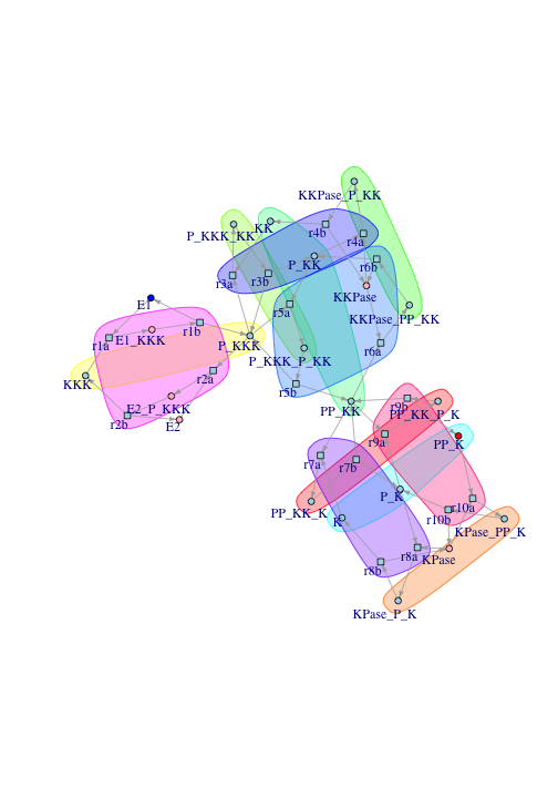
Looking more closely at the transition-invariants in this case:
transitions.sub <- transitions[!grepl("R", transitions)]
adjMat <- as.matrix(get.adjacency(subg))
pre <- adjMat[places, transitions.sub]
post <- t(adjMat[transitions.sub, places])
S <- post - pre
tInvariants <- getMinimalInvariants(t(S))
tInvariantsDescriptions <- lapply(tInvariants, function(tInv) mapk.nodes[tInv, "description"])
tInvariantsDescriptions


## [[1]]
## [1] "binding P-MAPKKK and P-MAPKK"    "phosphorylation of P-MAPKK"
## [3] "binding MAPKK-Pase and PP-MAPKK" "dephosphorylation of PP-MAPKK"
##
## [[2]]
## [1] "binding P-MAPKKK and MAPKK"     "phosphorylation of MAPKK"
## [3] "binding MAPKK-Pase and P-MAPKK" "dephosphorylation of P-MAPKK"
##
## [[3]]
## [1] "binding MAPK and PP-MAPKK"    "phosphorylation of MAPK"
## [3] "binding MAPK-Pase and P-MAPK" "dephosphorylation of P-MAPK"
##
## [[4]]
## [1] "binding of MAPKKK activator"   "MAPKKK activation"
## [3] "binding of MAPKKK inactivator" "MAPKKK inactivation"
##
## [[5]]
## [1] "binding PP-MAPKK and P-MAPK"   "phosphorylation of P-MAPK"
## [3] "binding MAPK-Pase and PP-MAPK" "dephosphorylation of PP-MAPK"
In the first cycle, once-phosphorylated Mek (P-MapKK) binds with phosphorylated Raf (P-MAPKKK), which leads to Mek taking on another phosphorylation. Then Mek phosphatase binds to the twice-phosphorylated Mek, leading to a dephosphorylation that takes Mek back to where it started. The other cycles have similar interpretations.
Combining Shortest Path with Subnetwork Approach
Since all the reactions in the shortest path fall in a transition-invariant, I can remove the reactions and just look at species:
spMat <- get.edgelist(g)[sp, ]
transitions <- V(g)[V(g)$type == "transition"]$name
transition.outgoing.mat <- spMat[spMat[, 1] %in% transitions, ]
transition.outgoing.list <- as.list(transition.outgoing.mat[, 2])
names(transition.outgoing.list) <- transition.outgoing.mat[, 1]
transition.incoming.mat <- spMat[spMat[, 2] %in% transitions, ]
transition.incoming.list <- as.list(transition.incoming.mat[, 1])
names(transition.incoming.list) <- transition.incoming.mat[, 2]
place.only.edges <- do.call("rbind", sapply(transitions, function(tr){
   c(from = transition.incoming.list[[tr]], to = transition.outgoing.list[[tr]])
}))
place.only.graph <- graph.edgelist(place.only.edges)
simple.layout <- matrix(c(20, 82, 165, 228, 309, 381, 430,
                          410, 329, 290, 208, 163, 95, 0), ncol = 2)
plot.igraph(place.only.graph, layout=simple.layout,
            vertex.size =4, vertex.label.dist=-.37,
            edge.arrow.size=.4 )
Finally, I go from referring to species to referring to super-nodes (place-invariants).
invariant.edges <- cbind(
  sapply(place.only.edges[, 1], function(place){
    out <- names(pInvariants)[sapply(pInvariants, function(inv) place %in% inv)]
    if(length(out) == 0) out <- place
    out
  }),
  sapply(place.only.edges[, 2], function(place){
    out <- names(pInvariants)[sapply(pInvariants, function(inv) place %in% inv)]
    if(length(out) == 0) out <- place
    out
  })
)
invariant.graph <- graph.edgelist(invariant.edges)
plot.igraph(invariant.graph, layout=simple.layout,
            vertex.size =4, vertex.label.dist=-.37,
            edge.arrow.size=.4 )
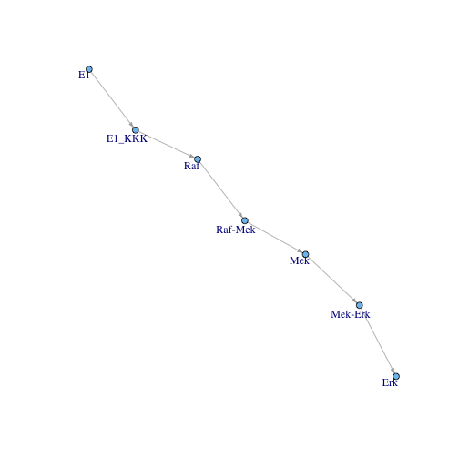
Conclusion
The best way to view the signal is to plot paths through subnetworks. The subnetworks are derived from invariant analysis.
References
Huang, Chi-Ying and James E. Ferrell. “Ultrasensitivity in the mitogen-activated protein kinase cascade.” Proceedings of the National Academy of Sciences 93.19 (1996): 10078-10083.
Sackmann, Andrea, Monika Heiner, and Ina Koch. “Application of Petri net based analysis techniques to signal transduction pathways.” BMC bioinformatics 7.1 (2006): 482.
Hardy, Simon and Ravi Iyengar. Analysis of Dynamic Models of Signaling Networks with Petri Nets and Dynamic Graphs. In Ina Koch, Wolfgang Reisig, and Falk Schreiber. Modeling in systems biology: the Petri Net approach. Vol. 16. Springer, (2010) (pp. 225-250).