Visualizing Performance In Bayesian Network Structure Learning
The bnlearn package helps you learn Bayesian networks from data. It has handy functions for plotting performance of Bayesian network structure learning.
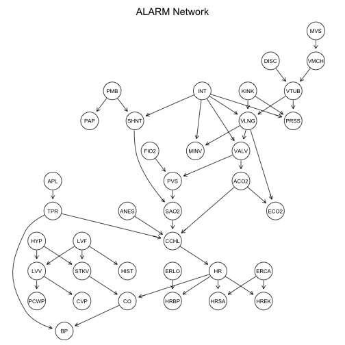
Below I demonstrate some network learnings performance visualizations on the ALARM network, a commonly used benchmark:
library(magrittr)
library(plyr)
library(dplyr)
library(bnlearn)

alarm.model.string <- paste("[HIST|LVF][CVP|LVV][PCWP|LVV][HYP][LVV|HYP:LVF]",
  "[LVF][STKV|HYP:LVF][ERLO][HRBP|ERLO:HR][HREK|ERCA:HR][ERCA]",
  "[HRSA|ERCA:HR][ANES][APL][TPR|APL][ECO2|ACO2:VLNG][KINK]",
  "[MINV|INT:VLNG][FIO2][PVS|FIO2:VALV][SAO2|PVS:SHNT][PAP|PMB][PMB]",
  "[SHNT|INT:PMB][INT][PRSS|INT:KINK:VTUB][DISC][MVS][VMCH|MVS]",
  "[VTUB|DISC:VMCH][VLNG|INT:KINK:VTUB][VALV|INT:VLNG][ACO2|VALV]",
  "[CCHL|ACO2:ANES:SAO2:TPR][HR|CCHL][CO|HR:STKV][BP|CO:TPR]", sep = "")
alarm.net <- alarm %>%
  names %>%
  empty.graph %>%
  `modelstring<-`(value = alarm.model.string)
graphviz.plot(alarm.net, main = "ALARM Network")
Using model averaging and the strength.plot function, I can get a visualization of the proportion of times each arc in the true network appeared in the model averaging bootstrap simulation. This is shown as edge thickness.
model.averaging <- boot.strength(data = alarm,
                                 R = 50, m = 100,
                                 algorithm = "hc",
                                 algorithm.args = list(score = "bde", iss = 10))
strength.plot(alarm.net, model.averaging)
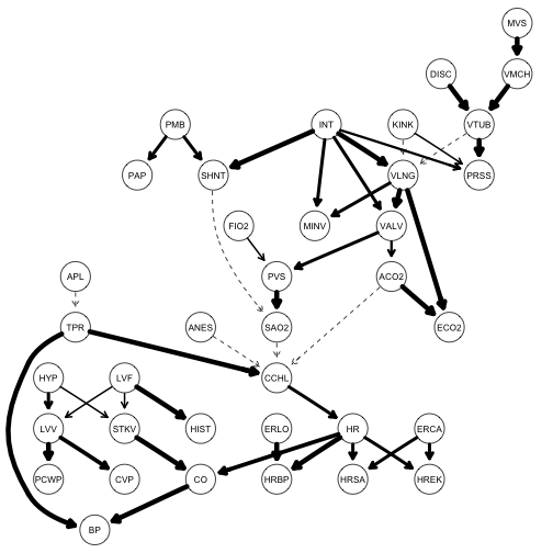
This reflects how well the network inference learned the true arcs – the thicker the arc, the more evidence the learning algorithm found in the data.
Similarly, I get a consensus network - a learned network created from the results of the model averaging, and visualize the evidence for each arc in the consensus network. The averaged.network function provides a consensus network from the averaging results, the threshold value is a cutoff – the arc must have appeared more than this percentage of times in the averaging samples. I set it very low so we can get lots of weak edges in the visualization.
consensus.net <- averaged.network(model.averaging, threshold = .01)
strength.plot(consensus.net, model.averaging)

Since the cutoff is so low, the network is thick with weak-evidence arcs.
ROC Curves
ROC curves are a classic visualization of learning performance. However, they are tricky in this case because they require a false positive rate. False positives are easy to get with the compare function:
compare(alarm.net, consensus.net)

## $tp
## [1] 22
##
## $fp
## [1] 390
##
## $fn
## [1] 24
However, the false positive rate is (FP / N), where N here is defined as “wrong arcs”, i.e. all the arcs that are not in the ALARM network. That means counting all the possible directed edges in graph. Since it is a directed acyclic graph, the presence of an edge depends on the presence of others, so this is a non-trivial problem.
An alternative is to convert the graph to a moral graph, where undirected edges represent conditional dependencies.
graphviz.plot(moral(alarm.net))
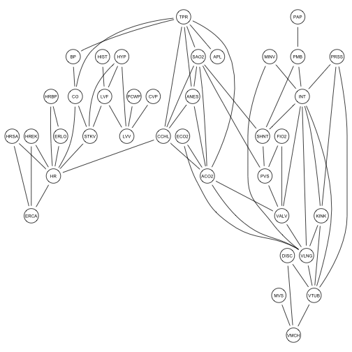
In this case, N is just the number of conditional independencies, which we can count – it is just the number of possible undirected edges ( n(n-1)/ 2, n = # nodes) minus the number of undirected edges in moral(alarm.net). The compare function still works with moral graphs.
compare(moral(alarm.net), moral(consensus.net))

## $tp
## [1] 65
##
## $fp
## [1] 573
##
## $fn
## [1] 0
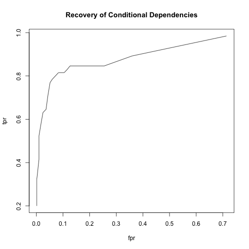
So we can get an ROC curve that reflects how well we recover not arcs, but the conditional dependences that the arcs determine.
I wrote a function that gives me true positive rate and false positive rate, and plotted an ROC curve. The main argument is the cutoff, which is passed as the threshold value in averaged.network. With different values of cutoff, I get different pairs of rates, giving me values to plot for the ROC curve.
getROCStats <- function(cutoff, true, model.averaging){
  consensus.net <- averaged.network(model.averaging, threshold = cutoff) %>%
    suppressWarnings
  pos <- narcs(moral(alarm.net))
  neg <- nnodes(alarm.net) %>%
    {.*(. - 1) / 2 - pos}
  compare(moral(alarm.net), moral(consensus.net)) %>%
    unlist %>%
    {c(.["tp"] / pos, .["fp"]/ neg)} %>%
    `names<-`(c("tpr", "fpr"))
}
adply(seq(.05, 1, by = .05), 1, getROCStats, true = alarm.net, model.averaging = model.averaging) %>%
  select(fpr, tpr) %>%
  plot(main = "Recovery of Conditional Dependencies", type = "l")